Database Optimization: From Query Tuning to Sharding - The Complete Guide
The Slow Query That Brought Down Production
It started as a simple report. "Show me all orders from the last month with customer details." The query worked fine in development with 1,000 rows. In production, with 50 million rows, it brought the entire application to its knees. Response times jumped from milliseconds to minutes. The connection pool exhausted. Users saw timeout errors.
This is the story of almost every scaling challenge. What works at small scale breaks catastrophically at large scale. Database optimization isn't about making things faster. It's about understanding why things are slow and choosing the right solution for your specific problem.
This guide covers everything from basic query optimization to advanced sharding strategies. More importantly, it explains when to use each technique and the trade-offs involved.
Understanding Why Databases Slow Down
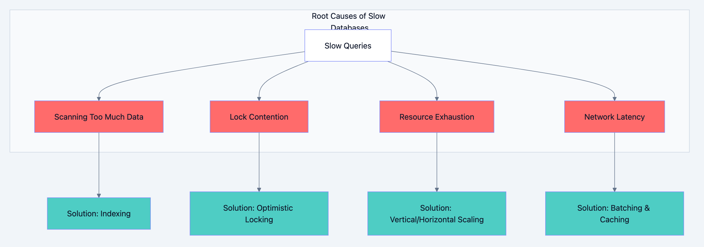
Before optimizing, you need to understand what causes slowness. Databases slow down for four fundamental reasons:
1. Scanning Too Much Data
When a query reads millions of rows to return ten results, you have a scanning problem. The database does more work than necessary. This happens with missing indexes, poor query design, or selecting unnecessary columns.
2. Lock Contention
Multiple transactions fighting for the same rows create waiting. While one transaction holds a lock, others queue up. High contention means high latency, even if individual operations are fast.
3. Resource Exhaustion
CPU, memory, disk I/O, or network bandwidth hitting limits. When the database server runs out of resources, everything slows down regardless of query quality.
4. Network Latency
Round trips between application and database add up. A query that makes 100 small database calls suffers more from network latency than one that makes a single call returning the same data.
Database optimization diagram 1
Query Optimization: The Foundation
Query optimization is your first line of defense. Before adding infrastructure, make sure your queries aren't wasteful.
The EXPLAIN Command: Your Diagnostic Tool
Every database has an EXPLAIN command that shows how queries execute. Learn to read it.
sqlEXPLAIN ANALYZE SELECT * FROM orders
WHERE customer_id = 12345
AND created_at > '2024-01-01';
The output tells you:
- Scan type: Sequential scan (bad for large tables) vs Index scan (good)
- Rows examined: How many rows the database looked at
- Execution time: Actual time spent
A query examining 10 million rows to return 100 results is a red flag. You're paying for work that produces no value.
Select Only What You Need
The most common mistake is
SELECT *. It seems convenient but causes real problems.Why SELECT * Hurts Performance:
First, you transfer more data over the network than necessary. A table with 50 columns sends 50 columns when you need 3. Second, you prevent covering indexes from working. A covering index contains all columns needed for a query, eliminating the need to read the actual table. With
SELECT *, no index can cover your query.Third, and most subtle,
SELECT * breaks when schemas change. Adding a column to a table suddenly increases payload size for all queries, even those that don't need the new column.sql-- Bad: Fetches all columns, prevents covering indexes SELECT * FROM users WHERE status = 'active'; -- Good: Only fetches needed columns, can use covering index SELECT id, name, email FROM users WHERE status = 'active';
Write Queries That Use Indexes
Indexes are useless if your queries can't use them. Several patterns prevent index usage:
Functions on indexed columns:
sql-- Cannot use index on created_at
SELECT * FROM orders WHERE YEAR(created_at) = 2024;

-- Can use index on created_at
SELECT * FROM orders WHERE created_at >= '2024-01-01' AND created_at < '2025-01-01';
Implicit type conversion:
sql-- If user_id is integer, this may not use index
SELECT * FROM orders WHERE user_id = '12345';

-- Correct type, uses index
SELECT * FROM orders WHERE user_id = 12345;
Leading wildcards:
sql-- Cannot use index (starts with wildcard)
SELECT * FROM products WHERE name LIKE '%phone%';

-- Can use index (wildcard at end only)
SELECT * FROM products WHERE name LIKE 'phone%';
OR conditions on different columns:
sql-- May not use indexes efficiently
SELECT * FROM users WHERE email = 'test@example.com' OR phone = '555-1234';

-- Better: Use UNION for each condition
SELECT * FROM users WHERE email = 'test@example.com'
UNION
SELECT * FROM users WHERE phone = '555-1234';
Avoid N+1 Query Problems
The N+1 problem happens when you fetch a list, then make one query per item in the list.
go// Bad: N+1 queries (1 for orders + N for customers)
orders := db.Query("SELECT * FROM orders LIMIT 100")
for _, order := range orders {
    customer := db.Query("SELECT * FROM customers WHERE id = ?", order.CustomerID)
    // process...
}

// Good: 2 queries total using JOIN or IN clause
orders := db.Query(`
    SELECT o.*, c.name, c.email
    FROM orders o
    JOIN customers c ON o.customer_id = c.id
    LIMIT 100
`)
The first approach makes 101 database round trips. The second makes 1. At scale, this difference is catastrophic.
Indexing Strategies: The Art of Fast Lookups
Indexes are data structures that speed up data retrieval at the cost of slower writes and additional storage. Understanding when and how to use them separates competent developers from database experts.
How Indexes Work
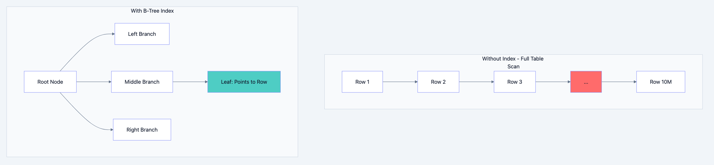
Think of an index like a book's index. Instead of reading every page to find mentions of "database," you look up "database" in the index, which points you directly to pages 42, 156, and 289.
Database indexes work similarly. A B-tree index (the most common type) maintains a sorted structure that allows finding any value in O(log n) time instead of O(n) time. For a table with 10 million rows, this means ~23 comparisons instead of 10 million.
Database optimization diagram 2
Types of Indexes
B-Tree Index (Default)
Best for: Equality comparisons, range queries, sorting. This is your default choice for most columns.
sqlCREATE INDEX idx_orders_customer ON orders(customer_id);
CREATE INDEX idx_orders_date ON orders(created_at);
Hash Index
Best for: Exact equality only. Faster than B-tree for equality but cannot help with ranges or sorting.
sql-- Only useful for: WHERE email = 'exact@match.com'
-- Cannot help with: WHERE email LIKE 'john%' or ORDER BY email
CREATE INDEX idx_users_email ON users USING HASH (email);
Composite Index (Multi-Column)
Best for: Queries filtering or sorting on multiple columns. Column order matters significantly.
sql-- Order matters! This index helps queries that filter by customer_id,
-- or customer_id AND status, or customer_id AND status AND created_at.
-- It does NOT help queries filtering only by status or only by created_at.
CREATE INDEX idx_orders_composite ON orders(customer_id, status, created_at);
The leftmost prefix rule means the index is useful only when you filter starting from the leftmost column. Think of it like a phone book sorted by last name, then first name. You can look up "Smith" or "Smith, John" but not just "John."
Covering Index
A covering index includes all columns a query needs, eliminating the need to read the actual table.
sql-- If most queries only need id, status, and amount:
CREATE INDEX idx_orders_covering ON orders(customer_id, status, created_at)
INCLUDE (id, amount);

-- This query can be satisfied entirely from the index:
SELECT id, status, amount FROM orders
WHERE customer_id = 123 AND status = 'pending';
Partial Index
Index only rows that match a condition. Smaller index, faster maintenance.
sql-- Only index active users (maybe 10% of total)
CREATE INDEX idx_active_users ON users(email) WHERE status = 'active';
When NOT to Index
Indexes aren't free. Every index:
- Slows down INSERT, UPDATE, DELETE operations
- Consumes storage space
- Requires maintenance during data modifications
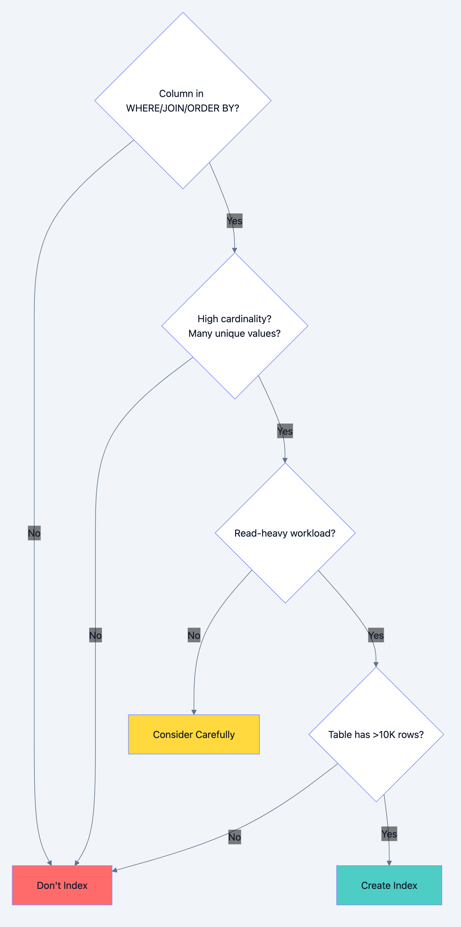
Don't index when:
-
Low cardinality columns: A boolean column with only true/false values won't benefit much from indexing. The database might scan half the table anyway.
-
Frequently updated columns: If a column changes constantly, the index maintenance overhead may exceed the query benefit.
-
Small tables: Tables with fewer than a few thousand rows often perform better with full scans than index lookups.
-
Write-heavy workloads: If you write 1000 times for every read, indexes hurt more than help.
Database optimization diagram 3
Caching: The Fastest Query Is No Query
The fastest database query is the one you don't make. Caching stores frequently accessed data in faster storage, reducing database load.
Caching Layers
Application-Level Cache (In-Memory)
Fastest but limited to single instance. Data lost on restart.
go// Simple in-memory cache
var userCache = make(map[int]*User)
var cacheMutex sync.RWMutex

func GetUser(id int) (*User, error) {
    // Check cache first
    cacheMutex.RLock()
    if user, ok := userCache[id]; ok {
        cacheMutex.RUnlock()
        return user, nil
    }
    cacheMutex.RUnlock()

    // Cache miss: query database
    user, err := db.QueryUser(id)
    if err != nil {
        return nil, err
    }

    // Store in cache
    cacheMutex.Lock()
    userCache[id] = user
    cacheMutex.Unlock()

    return user, nil
}
Distributed Cache (Redis/Memcached)
Shared across application instances. Survives individual server restarts. Network latency (~1ms) but much faster than database (~10-100ms).
Database Query Cache
Built into most databases. Automatically caches query results. Invalidated when underlying data changes. Useful for read-heavy, rarely-changing data.
Cache Invalidation Strategies
Cache invalidation is famously one of the two hard problems in computer science. Three main strategies exist:
Time-To-Live (TTL)
Data expires after a set duration. Simple but may serve stale data.
go// Set with 5 minute expiration
redis.Set("user:123", userData, 5*time.Minute)
Write-Through
Update cache whenever database updates. Always consistent but slower writes.
gofunc UpdateUser(user *User) error {
    // Update database
    err := db.UpdateUser(user)
    if err != nil {
        return err
    }

    // Update cache immediately
    redis.Set(fmt.Sprintf("user:%d", user.ID), user, 0)
    return nil
}
Write-Behind (Write-Back)
Update cache immediately, persist to database asynchronously. Fast writes but risk of data loss.
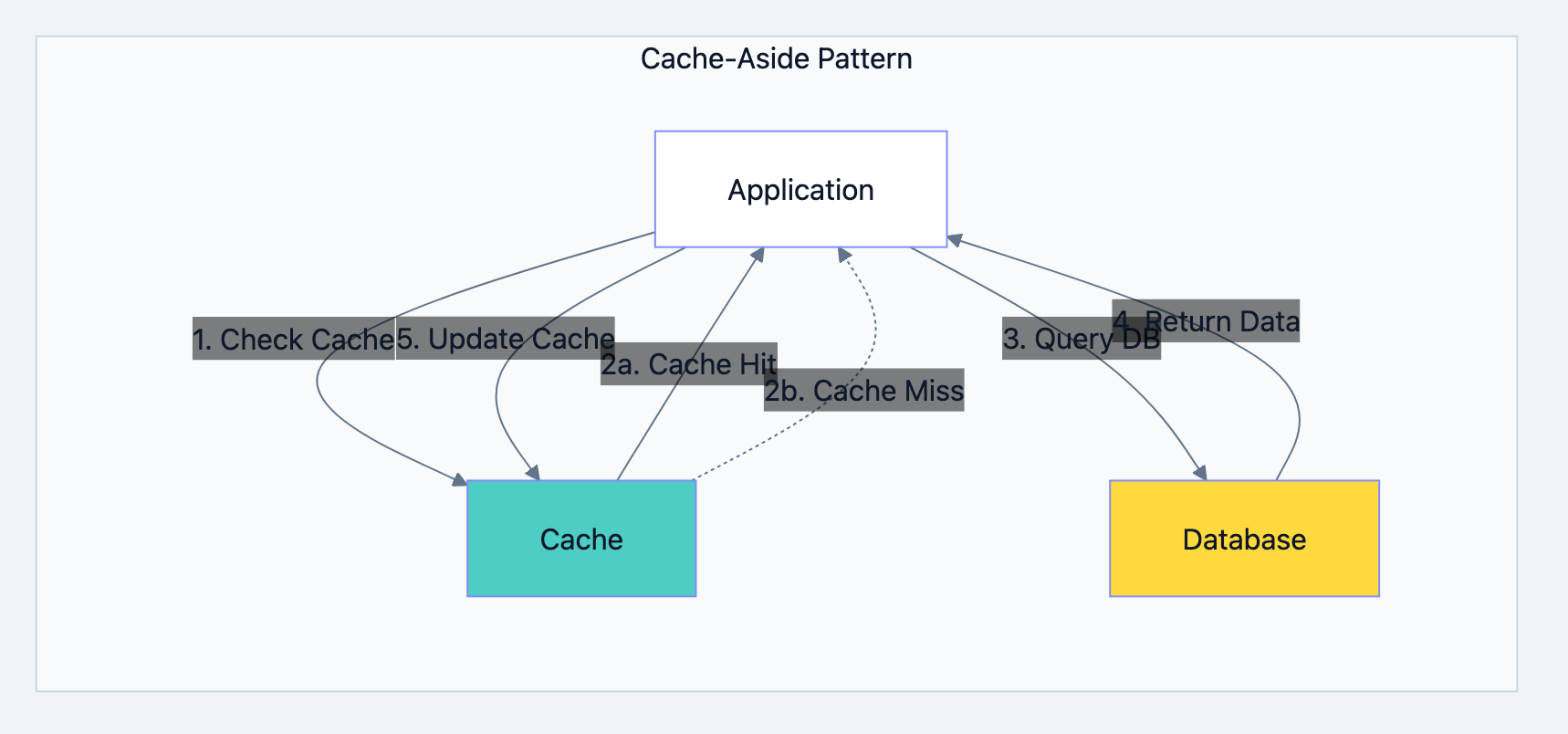
Cache-Aside (Lazy Loading)
Application manages cache. Read from cache, fall back to database, populate cache on miss.
Database optimization diagram 4
When to Cache
Cache when:
- Data is read frequently, written rarely
- Slight staleness is acceptable
- Computation to generate data is expensive
- Database is a bottleneck
Don't cache when:
- Data must always be current (financial transactions)
- Data is unique per request (already cacheable by nature)
- Write frequency exceeds read frequency
Replication: Read Scaling and High Availability
Replication copies data across multiple database servers. It serves two purposes: handling more read traffic and surviving server failures.
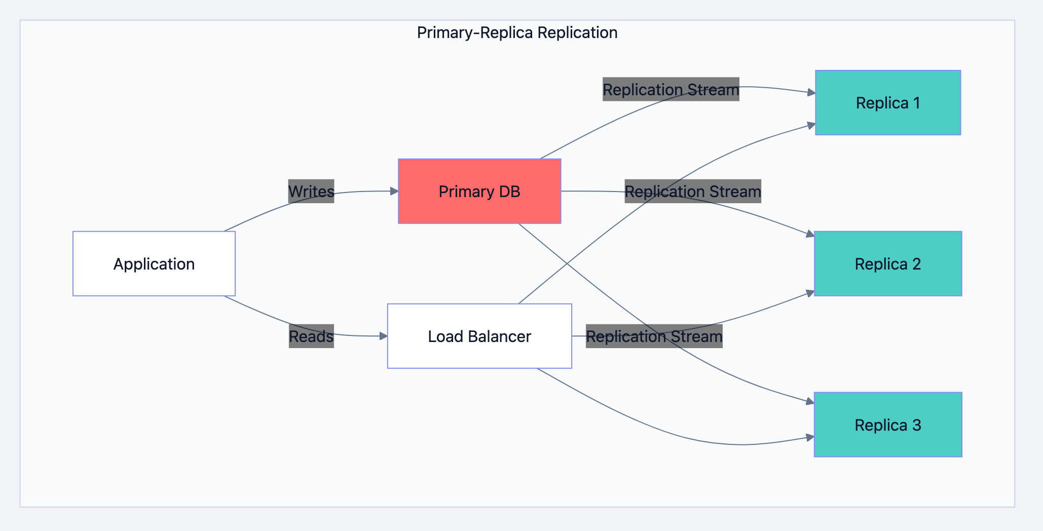
Primary-Replica Architecture
One primary server handles all writes. Multiple replicas receive copies and handle reads.
Database optimization diagram 5
Benefits:
- Read capacity scales horizontally (add more replicas)
- Primary failure doesn't lose data (promote a replica)
- Replicas can serve different purposes (reporting, analytics)
Trade-offs:
- Replication lag means replicas may have stale data
- Writes don't scale (still limited by primary)
- Complexity in handling failover and split-brain scenarios
Synchronous vs Asynchronous Replication
Synchronous Replication
Primary waits for replicas to confirm before acknowledging write. Guarantees no data loss but adds latency.
Write Request → Primary → Replica Confirms → Response to Client
Use when: Data loss is unacceptable (financial systems)
Asynchronous Replication
Primary acknowledges immediately, replicas catch up later. Lower latency but risk of data loss if primary fails before replication.
Write Request → Primary → Response to Client
                     ↓
              Replica (eventually)
Use when: Performance matters more than guaranteed durability
Handling Replication Lag
When a user writes data and immediately reads it, they might hit a replica that hasn't received the write yet. Solutions:
Read-Your-Writes Consistency
After writing, read from primary for a short period.
gofunc GetOrder(orderID int, justCreated bool) (*Order, error) {
    if justCreated {
        return db.Primary.Query("SELECT * FROM orders WHERE id = ?", orderID)
    }
    return db.Replica.Query("SELECT * FROM orders WHERE id = ?", orderID)
}
Monotonic Reads
Track the latest read position and ensure subsequent reads don't go backward.
Causal Consistency
If operation B depends on operation A, ensure B sees A's results.
Partitioning: Dividing Data for Manageability
Partitioning splits a large table into smaller pieces. Unlike sharding (which distributes across servers), partitioning typically keeps all partitions on the same server but in separate storage units.
Types of Partitioning
Range Partitioning
Split by value ranges. Common for time-series data.
sql-- Partition orders by year
CREATE TABLE orders (
    id BIGINT,
    customer_id INT,
    created_at TIMESTAMP,
    amount DECIMAL
) PARTITION BY RANGE (YEAR(created_at)) (
    PARTITION p2022 VALUES LESS THAN (2023),
    PARTITION p2023 VALUES LESS THAN (2024),
    PARTITION p2024 VALUES LESS THAN (2025),
    PARTITION p_future VALUES LESS THAN MAXVALUE
);
Benefits: Easy to drop old data (just drop partition), queries on date ranges scan fewer partitions.
List Partitioning
Split by explicit value lists. Good for categorical data.
sql-- Partition by region
CREATE TABLE customers (
    id INT,
    name VARCHAR(100),
    region VARCHAR(20)
) PARTITION BY LIST (region) (
    PARTITION p_north VALUES IN ('NY', 'MA', 'CT'),
    PARTITION p_south VALUES IN ('FL', 'GA', 'TX'),
    PARTITION p_west VALUES IN ('CA', 'WA', 'OR')
);
Hash Partitioning
Distribute evenly using hash function. Prevents hotspots but makes range queries expensive.
sql-- Distribute users evenly across 8 partitions
CREATE TABLE users (
    id INT,
    email VARCHAR(100)
) PARTITION BY HASH (id) PARTITIONS 8;
When to Partition
Partition when:
- Tables exceed hundreds of millions of rows
- You need to efficiently delete old data
- Queries naturally filter by partition key
- Maintenance operations (backups, index rebuilds) take too long
Don't partition when:
- Tables are small enough to manage as single units
- Queries frequently span all partitions
- You'd create thousands of tiny partitions
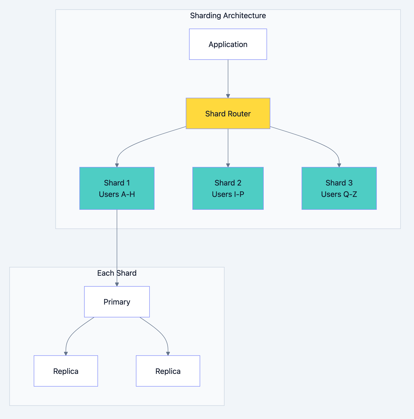
Sharding: Horizontal Scaling for Massive Data
Sharding distributes data across multiple database servers. Each server (shard) holds a portion of the total data. This is how you scale writes and storage beyond what a single server can handle.
Sharding Strategies
Range-Based Sharding
Assign ranges of keys to different shards.
Shard 1: user_id 1 - 1,000,000
Shard 2: user_id 1,000,001 - 2,000,000
Shard 3: user_id 2,000,001 - 3,000,000
Pros: Simple to understand, range queries stay on single shard
Cons: Uneven distribution (new users concentrate on latest shard), requires rebalancing as data grows
Hash-Based Sharding
Use hash function to determine shard.
gofunc GetShard(userID int, numShards int) int {
    return hash(userID) % numShards
}
Pros: Even distribution, no hotspots
Cons: Range queries must hit all shards, adding shards requires rehashing everything
Directory-Based Sharding
Lookup table maps keys to shards.
user_id 123 → Shard 2
user_id 456 → Shard 1
user_id 789 → Shard 3
Pros: Flexible placement, easy to move specific users
Cons: Lookup table becomes bottleneck/single point of failure
Geographic Sharding
Shard by user location for lower latency.
US users → US data center
EU users → EU data center
Asia users → Asia data center
Pros: Lower latency, data sovereignty compliance
Cons: Cross-region queries are slow, users who travel see latency spikes
Database optimization diagram 6
Sharding Challenges
Cross-Shard Queries
Queries spanning multiple shards are expensive. A simple JOIN becomes a distributed operation.
sql-- If users and orders are on different shards, this is painful
SELECT u.name, o.total
FROM users u
JOIN orders o ON u.id = o.user_id;
Solution: Co-locate related data. If you shard by user_id, put all of a user's data (orders, addresses, preferences) on the same shard.
Cross-Shard Transactions
Atomic transactions across shards require distributed transaction protocols (2-phase commit), which are slow and complex.
Solution: Design to avoid cross-shard transactions. Use eventual consistency where possible.
Rebalancing
As data grows unevenly or you add shards, you must move data between shards without downtime.
Solution: Use consistent hashing to minimize data movement when adding/removing shards.
Operational Complexity
Every operation (backups, upgrades, monitoring) multiplies by number of shards.
When to Shard
Shard when:
- Single database can't handle write volume
- Data size exceeds single server storage
- You need geographic distribution
- Vertical scaling (bigger server) is cost-prohibitive
Don't shard when:
- Read replicas can handle your load
- Partitioning solves your problem
- Your data fits on one server with room to grow
- You haven't exhausted simpler optimizations
Warning: Sharding is expensive to implement and maintain. Most applications never need it. Premature sharding adds complexity without benefit.
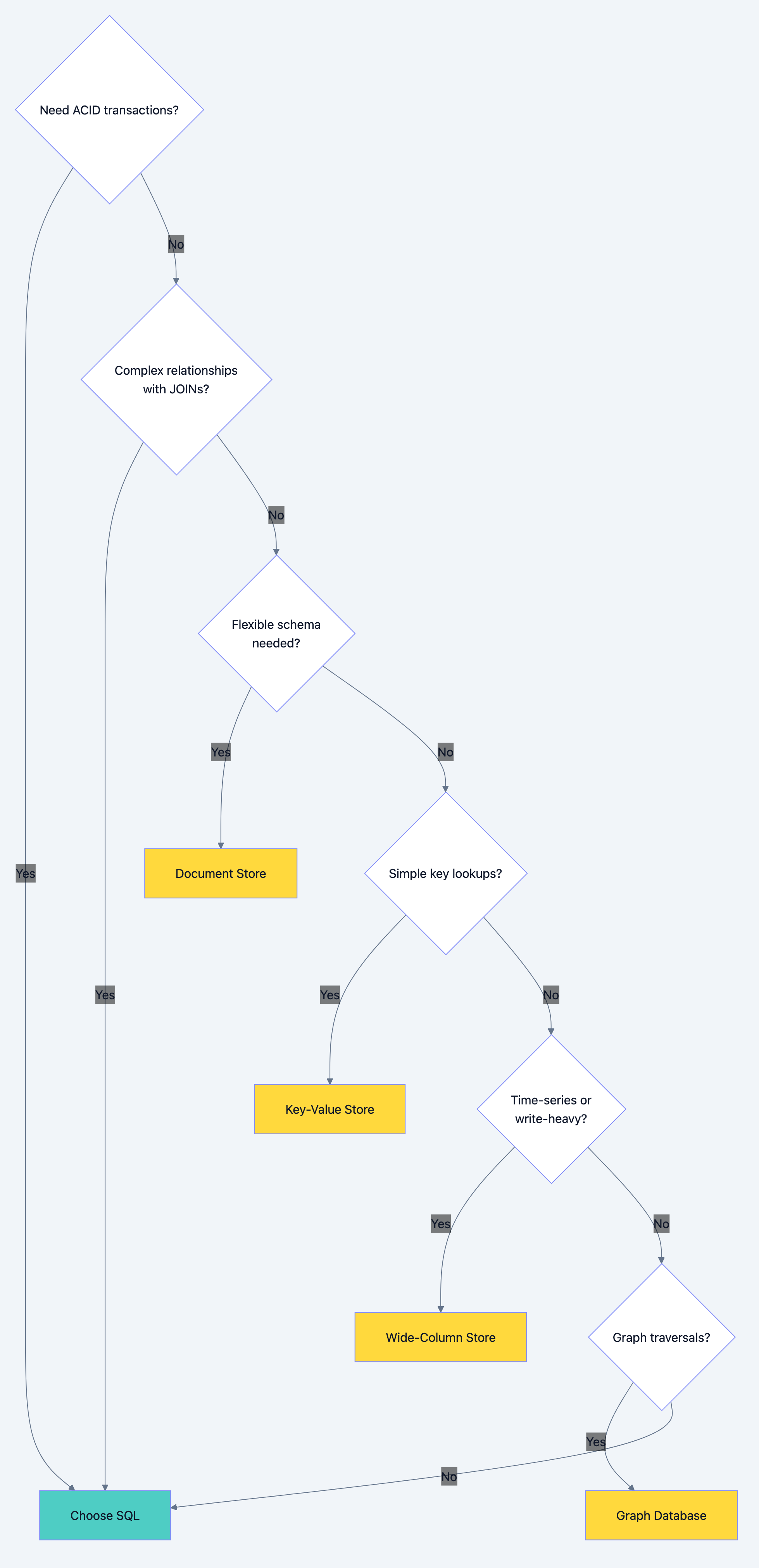
SQL vs NoSQL: Choosing the Right Database
The SQL vs NoSQL debate misses the point. Each has use cases where it excels. Understanding the trade-offs lets you choose correctly.
When to Choose SQL (Relational Databases)
Strong Consistency Required
Financial transactions, inventory management, booking systems. When you can't afford to oversell or double-book, SQL's ACID transactions are essential.
Complex Relationships
Data with many relationships (users have orders, orders have items, items have categories, categories have hierarchies). Relational databases excel at JOINs.
Ad-hoc Queries
Business analysts running arbitrary queries. SQL's query language handles complex aggregations, filters, and groupings that are painful in NoSQL.
Schema Stability
Data structure is well-understood and unlikely to change dramatically. Relational schemas enforce data integrity.
Examples: E-commerce, banking, ERP systems, traditional business applications.
When to Choose NoSQL
Document Stores (MongoDB, CouchDB)
Use for: Flexible schemas, hierarchical data, content management
Example: Blog posts with varying structures, product catalogs with different attributes per category
json{
    "type": "laptop",
    "brand": "Apple",
    "specs": {
        "cpu": "M2",
        "ram": "16GB",
        "storage": "512GB"
    },
    "reviews": [...]
}
Key-Value Stores (Redis, DynamoDB)
Use for: Caching, session storage, simple lookups
Example: User sessions, feature flags, rate limiting counters
session:abc123 → {user_id: 456, expires: 1709251200}
ratelimit:user:789 → 47
Wide-Column Stores (Cassandra, HBase)
Use for: Time-series data, write-heavy workloads, massive scale
Example: IoT sensor data, event logs, activity feeds
Graph Databases (Neo4j, Amazon Neptune)
Use for: Highly connected data, relationship-heavy queries
Example: Social networks, recommendation engines, fraud detection
Database optimization diagram 7
Scaling SQL Databases
SQL databases can scale, just differently:
- Read Replicas: Scale reads horizontally
- Connection Pooling: Handle more concurrent connections
- Partitioning: Manage large tables
- Sharding: Scale writes (with significant complexity)
- NewSQL: Databases like CockroachDB, TiDB provide SQL interface with horizontal scaling
Scaling NoSQL Databases
NoSQL typically scales more naturally:
- Built-in Sharding: Most NoSQL databases shard automatically
- Eventual Consistency: Trade consistency for availability and partition tolerance
- Denormalization: Store data redundantly to avoid joins
- Horizontal Scaling: Add nodes to increase capacity
The trade-off: NoSQL sacrifices query flexibility and consistency for scaling simplicity.
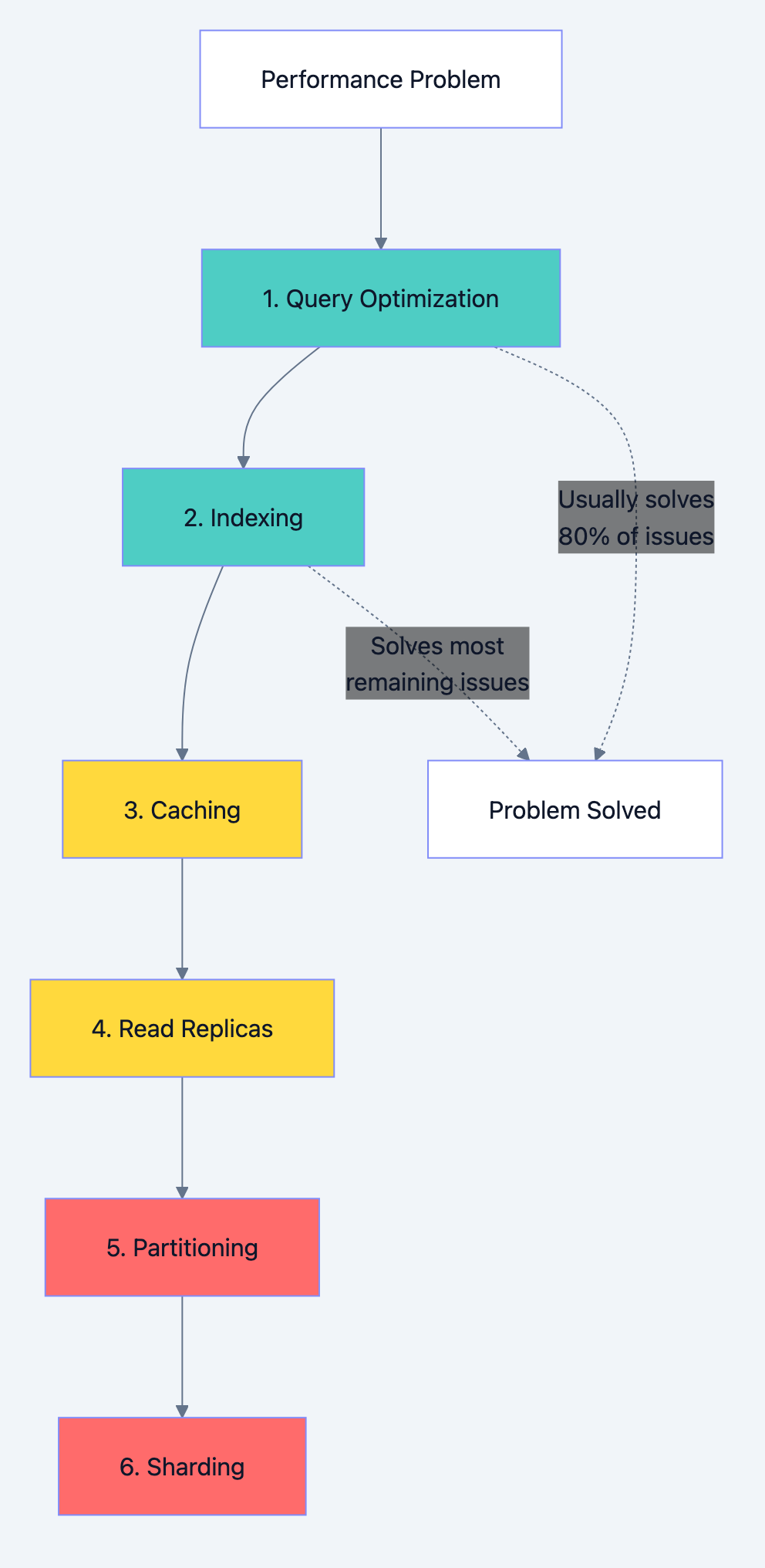
The Optimization Roadmap
When facing database performance issues, follow this order:
Database optimization diagram 8
Level 1: Query Optimization (Do This First)
- Use EXPLAIN to understand query execution
- Select only needed columns
- Eliminate N+1 queries
- Cost: Low. Benefit: Often 10-100x improvement.
Level 2: Indexing
- Add indexes for common query patterns
- Create composite indexes for multi-column filters
- Remove unused indexes
- Cost: Low-Medium. Benefit: 10-1000x for specific queries.
Level 3: Caching
- Cache frequently accessed, rarely changing data
- Implement proper invalidation strategies
- Cost: Medium. Benefit: 10-100x for cached data.
Level 4: Read Replicas
- Offload read traffic from primary
- Handle replication lag in application
- Cost: Medium-High. Benefit: Linear scaling of reads.
Level 5: Partitioning
- Split large tables into manageable pieces
- Align partitions with query patterns
- Cost: Medium. Benefit: Better maintenance, faster queries on partition key.
Level 6: Sharding
- Distribute data across multiple servers
- Significant application changes required
- Cost: Very High. Benefit: Horizontal scaling of writes and storage.
Common Mistakes to Avoid
Premature Optimization
Don't shard a database that handles 100 requests per second. Don't add 20 indexes "just in case." Optimize based on actual measurements, not imagined future load.
Ignoring the Obvious
A slow query might just need an index. Check the basics before architecting complex solutions.
Over-Caching
Caching everything creates cache invalidation nightmares. Cache selectively where it provides clear value.
Wrong Tool for the Job
Using MongoDB for financial transactions or PostgreSQL for social graph traversals. Match database type to access patterns.
Not Monitoring
You can't optimize what you don't measure. Track query performance, cache hit rates, replication lag, and resource utilization.
What You Learned
Database optimization is a progression, not a single technique:
- Query optimization eliminates wasteful work
- Indexing speeds up data retrieval
- Caching avoids queries entirely
- Replication scales read capacity
- Partitioning manages large tables
- Sharding scales write capacity and storage
- Database selection matches tool to problem
Most applications need only the first three levels. Reach for advanced techniques only when simpler solutions fail. Every optimization adds complexity. Choose the simplest solution that solves your actual problem.
Start with measurement. Understand where time goes. Then optimize systematically, validating improvements at each step. Database performance isn't magic. It's understanding the fundamentals and applying them correctly to your specific situation.