The Ultimate Coding Interview Cheatsheet: Master Pattern Recognition in 30 Minutes
The Panic Before the Interview
It's 9 AM. Your Google interview is in 30 minutes. You've solved 300 LeetCode problems, but as you sit there, your mind goes blank. "Was this a DP problem? Should I use a HashMap? Wait, is this even solvable in O(n)?"
You're not alone. The biggest challenge in coding interviews isn't knowing how to implement algorithms it's recognizing which technique to use in the first place. You have 45 minutes to solve a problem you've never seen before, and the first 5 minutes of pattern recognition determine whether you succeed or struggle.
This cheatsheet solves that problem. It's the mental framework that transforms you from "I hope I remember this" to "I know exactly what to do." Let's build that framework.
Why Interview Prep Feels Overwhelming
What Problem Does This Solve?
The core challenge: There are hundreds of data structures and dozens of algorithmic patterns. In an interview, you have minutes (not hours) to:
- Understand the problem
- Identify the right approach
- Choose the optimal data structure
- Code the solution
- Analyze time/space complexity
What existed before?
Traditionally, developers prepared by:
- Solving problems randomly (no pattern recognition)
- Memorizing solutions (doesn't transfer to new problems)
- Studying algorithms in isolation (can't map to real problems)
The limitations:
Random practice: Solving 500 problems without learning patterns means you're starting from zero on problem 501
Solution memorization: "I remember this problem used a HashMap" doesn't help when the problem is slightly different
Algorithm-first learning: Knowing how Dijkstra's algorithm works doesn't help you recognize when to use it
Why was a new approach needed?
Interviews test pattern recognition, not memorization. You need a mental framework that maps problem characteristics → technique in seconds.
![A[Traditional Approach] to B[Solve Random Problems]](/diagrams/coding-cheat-sheet/01-traditional-vs-pattern-approach.png)
A[Traditional Approach] to B[Solve Random Problems]
Real-World Analogy
Think of coding interviews like medical diagnosis:
- Patient symptoms = Problem description keywords
- Diagnostic patterns = Algorithmic patterns (two pointers, DP, etc.)
- Treatment = The solution you implement
A doctor doesn't memorize every patient they've ever seen. They learn to recognize patterns:
- "Fever + cough + fatigue" → Likely flu → Test and treat accordingly
- "Chest pain + shortness of breath" → Possible cardiac → Run ECG
Similarly, you learn to recognize:
- "Sorted array + target sum" → Two pointers
- "Optimal + overlapping subproblems" → Dynamic programming
- "All possible combinations" → Backtracking
The skill isn't memorization it's pattern recognition.
A Mental Framework for Pattern Recognition
How Does This Cheatsheet Solve the Problem?
Instead of memorizing 500 solutions, you'll learn:
- 12 core data structures and when to use each
- 10 algorithmic patterns that solve 90% of interview problems
- Keyword mapping from problem description to technique
- Complexity awareness to know when you've found the optimal solution
Key innovations:
Keyword-driven: Train your brain to see "sorted" and think "binary search"
Complexity-aware: Know the best possible time complexity to avoid over-optimization
Decision trees: Visual frameworks to choose the right approach in seconds
Anti-patterns: Learn what NOT to do (just as important)
High-Level Architecture
Here's how the framework works:
![A[Read Problem] to B[Extract Keywords]](/diagrams/coding-cheat-sheet/02-solution-framework.png)
A[Read Problem] to B[Extract Keywords]
Why this approach works:
- Speed: Keywords → Pattern mapping happens in seconds
- Reliability: Patterns work across hundreds of problems
- Confidence: You know when you've found the optimal solution
- Transferability: Patterns apply to problems you've never seen
The Pattern Recognition Framework
Building Your Mental Toolkit
Let's build a complete mental model of data structures, patterns, and how to choose between them.
Mental Model 1: Data Structure Decision Tree
![A[What operations do you need?] to B{Fast lookup/<br/>existe](/diagrams/coding-cheat-sheet/03-data-structure-decision-tree.png)
A[What operations do you need?] to B{Fast lookup/<br/>existe
How to use this:
When you read a problem, immediately ask: "What operations will I do most frequently?"
- Lookup/check existence → HashMap/HashSet
- Maintain sorted order → TreeSet/Heap
- Track min/max dynamically → Heap
- String prefix operations → Trie
- LIFO operations (undo, parsing) → Stack
- FIFO operations (BFS, task queue) → Queue
Mental Model 2: Pattern Recognition Flow
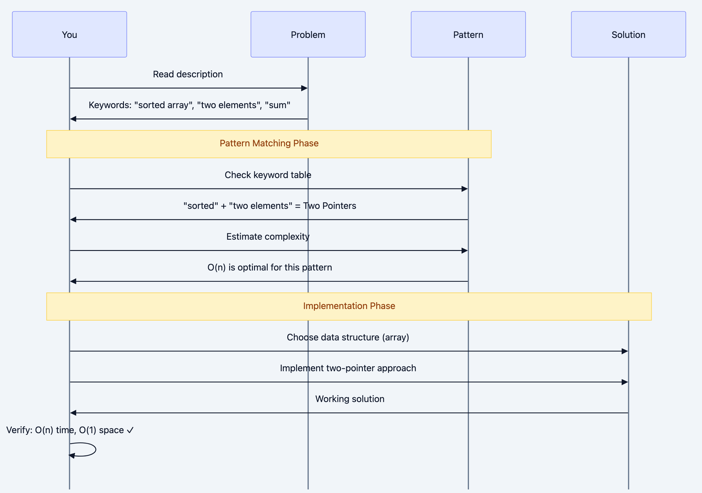
Sequence diagram 4
The mental checklist:
- Read and extract keywords (sorted, subarray, maximum, all possible)
- Map to pattern (use the keyword table below)
- Estimate best-case complexity (can this be O(n)? Must it be O(n²)?)
- Choose data structure (based on operations needed)
- Code and verify (check complexity matches estimate)
Mental Model 3: Time Complexity Awareness
Understanding what's possible vs. impossible is critical:
![A[Problem Characteristics] to B{Must examine<br/>all element](/diagrams/coding-cheat-sheet/05-complexity-awareness.png)
A[Problem Characteristics] to B{Must examine<br/>all element
Critical insight: If the problem requires examining all pairs (like finding duplicate in unsorted array), O(n²) might be optimal. Don't waste time searching for O(n) if it's impossible.
Mental Model 4: Pattern Decision Matrix
![[*] to ReadProblem](/diagrams/coding-cheat-sheet/06-pattern-state-machine.png)
[*] to ReadProblem
Deep Technical Dive: The Complete Toolkit
Part 1: Data Structures - When to Use What
Let's examine each data structure with the "What operations does this optimize?"
1. Array / Dynamic Array
Optimizes: Random access by index
Use when:
- Need O(1) access to any element
- Know the size upfront (array) or need dynamic resizing (ArrayList)
- Memory locality matters (cache-friendly)
Operations:
- Access: O(1)
- Search: O(n) unsorted, O(log n) sorted
- Insert/Delete at end: O(1) amortized
- Insert/Delete in middle: O(n)
Interview patterns:
- Two pointers
- Sliding window
- Binary search (if sorted)
2. HashMap / HashSet
Optimizes: Lookup, insertion, deletion
Use when:
- Need O(1) average-case lookup
- Tracking frequency/count
- Checking for duplicates
- Caching/memoization
Operations:
- Insert: O(1) average
- Lookup: O(1) average
- Delete: O(1) average
- Worst case (collisions): O(n)
Interview patterns:
- Counting frequencies
- Two sum variations
- Detect duplicates
- Cache/memoize recursive calls
go# Example: Two Sum using HashMap
func twoSum(nums []int, target int) []int {
	seen := make(map[int]int) // num -> index

	for i, num := range nums {
		complement := target - num

		// O(1) lookup - this is why we use HashMap
		if idx, ok := seen[complement]; ok {
			return []int{idx, i}
		}

		// Store for future lookups
		seen[num] = i
	}

	return []int{}
}
Why this works: Instead of O(n²) nested loop checking all pairs, we do single pass with O(1) lookups.
3. Stack
Optimizes: LIFO (Last In, First Out) access
Use when:
- Need to track "most recent" items
- Undo operations
- Matching pairs (brackets, tags)
- Recursion simulation (DFS)
- Monotonic problems
Operations:
- Push: O(1)
- Pop: O(1)
- Peek: O(1)
Interview patterns:
- Valid parentheses
- Next greater element
- Expression evaluation
- DFS (iterative)
gofunc validParentheses(s string) bool {
	stack := []rune{}
	// Map closing to opening brackets
	mapping := map[rune]rune{
		')': '(',
		'}': '{',
		']': '[',
	}

	for _, char := range s {
		if open, isClosing := mapping[char]; isClosing {
			// Check if it matches the most recent opening
			if len(stack) == 0 || stack[len(stack)-1] != open {
				return false
			}
			stack = stack[:len(stack)-1] // pop
		} else {
			// Opening bracket
			stack = append(stack, char)
		}
	}

	// Valid if all brackets matched (stack empty)
	return len(stack) == 0
}
Mental model: Stack = "undo buffer". Last thing added is first thing removed.
4. Queue / Deque
Optimizes: FIFO (First In, First Out) access
Use when:
- BFS traversal
- Sliding window (with deque)
- Task scheduling
- Level-order processing
Operations:
- Enqueue: O(1)
- Dequeue: O(1)
- Peek: O(1)
Interview patterns:
- BFS (shortest path, level-order)
- Sliding window maximum (deque)
- Design cache (LRU)
gofunc bfsShortestPath(graph map[string][]string, start, end string) []string {
	type NodePath struct {
		node string
		path []string
	}

	queue := []NodePath{{start, []string{start}}}
	visited := make(map[string]bool)
	visited[start] = true

	for len(queue) > 0 {
		// FIFO: process nodes level-by-level
		current := queue[0]
		queue = queue[1:]

		node := current.node
		path := current.path

		if node == end {
			return path
		}

		for _, neighbor := range graph[node] {
			if !visited[neighbor] {
				visited[neighbor] = true

				// Copy path to avoid mutation issues
				newPath := append([]string{}, path...)
				newPath = append(newPath, neighbor)

				queue = append(queue, NodePath{neighbor, newPath})
			}
		}
	}

	return []string{} // No path found
}
Why BFS uses Queue: FIFO ensures we explore all nodes at distance k before exploring distance k+1.
5. Heap (Priority Queue)
Optimizes: Access to min/max element
Use when:
- Need top K elements
- Dynamic min/max (elements added/removed)
- Merge K sorted arrays
- Median of stream
Operations:
- Insert: O(log n)
- Get min/max: O(1)
- Remove min/max: O(log n)
Interview patterns:
- Top K frequent elements
- Kth largest element
- Merge K sorted lists
- Median finder
gotype Item struct {
	num   int
	count int
}

// MinHeap implements heap.Interface for Item based on count
type MinHeap []Item

func (h MinHeap) Len() int            { return len(h) }
func (h MinHeap) Less(i, j int) bool  { return h[i].count < h[j].count } // min heap by count
func (h MinHeap) Swap(i, j int)       { h[i], h[j] = h[j], h[i] }
func (h *MinHeap) Push(x interface{}) { *h = append(*h, x.(Item)) }
func (h *MinHeap) Pop() interface{} {
	old := *h
	n := len(old)
	item := old[n-1]
	*h = old[:n-1]
	return item
}

// topKFrequent finds k most frequent elements
//
// Why Heap? Maintain top K elements efficiently
// Alternative: sort all (O(n log n)) - heap is O(n log k)
//
// Time: O(n log k)
// Space: O(n)
func topKFrequent(nums []int, k int) []int {
	// Count frequencies
	freq := make(map[int]int)
	for _, num := range nums {
		freq[num]++
	}

	h := &MinHeap{}
	heap.Init(h)

	for num, count := range freq {
		heap.Push(h, Item{num, count})

		// Keep only k elements
		if h.Len() > k {
			heap.Pop(h) // remove least frequent
		}
	}

	// Extract elements (ignore frequencies)
	result := []int{}
	for h.Len() > 0 {
		item := heap.Pop(h).(Item)
		result = append(result, item.num)
	}

	return result
}
Mental model: Heap = "automatic sorter for top K". Always gives you min/max in O(1).
6. Tree / Binary Search Tree
Optimizes: Hierarchical relationships, sorted access
Use when:
- Hierarchical data (file system, org chart)
- Range queries
- Sorted iteration (BST)
BST Operations (balanced):
- Search: O(log n)
- Insert: O(log n)
- Delete: O(log n)
- In-order traversal: O(n) - sorted order
Interview patterns:
- Validate BST
- Lowest common ancestor
- Serialize/deserialize
- Range sum queries
7. Trie (Prefix Tree)
Optimizes: Prefix operations on strings
Use when:
- Autocomplete
- Spell checker
- IP routing
- Dictionary operations
Operations:
- Insert word: O(m) where m = word length
- Search word: O(m)
- Search prefix: O(m)
go// TrieNode represents a node in the Trie
type TrieNode struct {
	children map[rune]*TrieNode // char -> TrieNode
	isEnd    bool               // End of word marker
}

// Trie represents the prefix tree
//
// Why Trie? O(m) prefix search vs O(n*m) scanning all words
// where m = word length, n = number of words
type Trie struct {
	root *TrieNode
}

// NewTrie initializes a Trie
func NewTrie() *Trie {
	return &Trie{
		root: &TrieNode{children: make(map[rune]*TrieNode)},
	}
}

// Insert inserts a word into the trie
// Time: O(m) where m = len(word)
func (t *Trie) Insert(word string) {
	node := t.root

	// Build path character by character
	for _, char := range word {
		if _, exists := node.children[char]; !exists {
			node.children[char] = &TrieNode{children: make(map[rune]*TrieNode)}
		}
		node = node.children[char]
	}

	node.isEnd = true // Mark end of word
}

// Search checks if a word exists
// Time: O(m)
func (t *Trie) Search(word string) bool {
	node := t.root

	for _, char := range word {
		if _, exists := node.children[char]; !exists {
			return false
		}
		node = node.children[char]
	}

	return node.isEnd
}

// StartsWith checks if any word starts with prefix
// Time: O(m) where m = len(prefix)
//
// This is THE reason to use Trie - O(m) prefix search
func (t *Trie) StartsWith(prefix string) bool {
	node := t.root

	for _, char := range prefix {
		if _, exists := node.children[char]; !exists {
			return false
		}
		node = node.children[char]
	}

	return true
}
Why Trie wins: For n words, average length m:
- Hash set search: O(m) but no prefix support
- Scanning all words: O(n*m) for prefix
- Trie: O(m) for both word and prefix search
8. Graph (Adjacency List)
Optimizes: Relationships between entities
Use when:
- Network connectivity
- Dependencies (task scheduling)
- Social networks
- Game boards (grid = graph)
Representations:
go# Adjacency List (most common in interviews)
graph := map[string][]string{
    "A": {"B", "C"},
    "B": {"A", "D"},
    "C": {"A"},
    "D": {"B"},
}


# Adjacency Matrix (for dense graphs)
# matrix[i][j] = 1 if edge exists
matrix := [][]int{
    {0, 1, 1, 0},
    {1, 0, 0, 1},
    {1, 0, 0, 0},
    {0, 1, 0, 0},
}
Interview patterns:
- BFS/DFS traversal
- Detect cycle
- Topological sort
- Shortest path (Dijkstra, BFS)
- Connected components
9. Union-Find (Disjoint Set)
Optimizes: Connected components, cycle detection
Use when:
- Find if two nodes are connected
- Count connected components
- Detect cycles in undirected graph
- Kruskal's MST
Operations (with path compression + union by rank):
- Find: O(α(n)) ≈ O(1) amortized
- Union: O(α(n)) ≈ O(1) amortized
gotype UnionFind struct {
	parent []int
	rank   []int
}

// NewUnionFind initializes DSU for n elements
func NewUnionFind(n int) *UnionFind {
	parent := make([]int, n)
	rank := make([]int, n)

	for i := 0; i < n; i++ {
		parent[i] = i // each node is its own parent initially
	}

	return &UnionFind{parent, rank}
}

// Find finds root of x with path compression
//
// Path compression makes operations nearly O(1) amortized
func (uf *UnionFind) Find(x int) int {
	if uf.parent[x] != x {
		uf.parent[x] = uf.Find(uf.parent[x])
	}
	return uf.parent[x]
}

// Union merges sets containing x and y
//
// Union by rank attaches smaller tree under larger tree
func (uf *UnionFind) Union(x, y int) bool {
	rootX := uf.Find(x)
	rootY := uf.Find(y)

	if rootX == rootY {
		return false // already connected
	}

	if uf.rank[rootX] < uf.rank[rootY] {
		uf.parent[rootX] = rootY
	} else if uf.rank[rootX] > uf.rank[rootY] {
		uf.parent[rootY] = rootX
	} else {
		uf.parent[rootY] = rootX
		uf.rank[rootX]++
	}

	return true
}

// Connected checks if x and y are in same set
func (uf *UnionFind) Connected(x, y int) bool {
	return uf.Find(x) == uf.Find(y)
}

// countComponents counts connected components in undirected graph
//
// Time: O(E * α(n)) ≈ O(E)
// Space: O(n)
func countComponents(n int, edges [][]int) int {
	uf := NewUnionFind(n)

	// Union all edges
	for _, edge := range edges {
		uf.Union(edge[0], edge[1])
	}

	// Count unique roots
	roots := make(map[int]bool)
	for i := 0; i < n; i++ {
		roots[uf.Find(i)] = true
	}

	return len(roots)
}
Part 2: Algorithmic Patterns - The Core 10
Pattern 1: Two Pointers
When to use: Sorted array, pairs/triplets, palindrome
Why it works: Reduces O(n²) nested loop to O(n) by intelligently moving pointers
Template:
def two_pointers_template(arr): """ Time: O(n) - single pass Space: O(1) - only pointers """ left, right = 0, len(arr) - 1 while left < right: # Check condition if condition_met(arr[left], arr[right]): return [left, right] elif need_larger_sum: left += 1 # Move left pointer right else: right -= 1 # Move right pointer left return []
Example: Three Sum
def three_sum(nums): """ Find all triplets that sum to zero Why Two Pointers? After fixing one number, two sum becomes sorted array problem Time: O(n²) - O(n) for each of n numbers Space: O(1) - ignoring output array """ nums.sort() # O(n log n) result = [] for i in range(len(nums) - 2): # Skip duplicates for first number if i > 0 and nums[i] == nums[i-1]: continue # Two pointers for remaining array left, right = i + 1, len(nums) - 1 target = -nums[i] # We want nums[i] + nums[left] + nums[right] = 0 while left < right: current_sum = nums[left] + nums[right] if current_sum == target: result.append([nums[i], nums[left], nums[right]]) # Skip duplicates while left < right and nums[left] == nums[left + 1]: left += 1 while left < right and nums[right] == nums[right - 1]: right -= 1 left += 1 right -= 1 elif current_sum < target: left += 1 # Need larger sum else: right -= 1 # Need smaller sum return result print(three_sum([-1, 0, 1, 2, -1, -4])) # [[-1,-1,2], [-1,0,1]]
Why this beats brute force:
- Brute force: O(n³) - check all triplets
- Two pointers: O(n²) - fix one, use two pointers for rest
Pattern 2: Sliding Window
When to use: Subarray/substring with constraint (max/min length, sum, distinct chars)
Why it works: Avoid recalculating from scratch by sliding window incrementally
Template:
def sliding_window_template(arr): """ Time: O(n) - each element enters/exits window once Space: O(1) or O(k) for window state """ left = 0 window_state = {} # Track window contents result = 0 for right in range(len(arr)): # Expand window: add arr[right] window_state[arr[right]] = window_state.get(arr[right], 0) + 1 # Shrink window while invalid while window_invalid(window_state): window_state[arr[left]] -= 1 left += 1 # Update result with current valid window result = max(result, right - left + 1) return result
Example: Longest Substring Without Repeating Characters
def length_of_longest_substring(s): """ Find length of longest substring without repeating characters Why Sliding Window? Instead of checking every substring O(n²), expand/contract window intelligently in O(n) Time: O(n) - each char enters and exits window once Space: O(min(n, m)) where m = charset size """ char_index = {} # char -> last seen index max_length = 0 left = 0 for right, char in enumerate(s): # If char repeats, move left past its last occurrence if char in char_index and char_index[char] >= left: left = char_index[char] + 1 # Update last seen index char_index[char] = right # Update max length max_length = max(max_length, right - left + 1) return max_length print(length_of_longest_substring("abcabcbb")) # 3 ("abc") print(length_of_longest_substring("bbbbb")) # 1 ("b") print(length_of_longest_substring("pwwkew")) # 3 ("wke")
Mental model: Window = "elastic band". Expand right, shrink left when invalid.
Pattern 3: Binary Search
When to use: Sorted array, search space can be halved, monotonic function
Why it works: Eliminates half of search space each iteration → O(log n)
Template:
def binary_search_template(arr, target): """ Time: O(log n) - halve search space each iteration Space: O(1) """ left, right = 0, len(arr) - 1 while left <= right: mid = left + (right - left) // 2 # Avoid overflow if arr[mid] == target: return mid elif arr[mid] < target: left = mid + 1 # Search right half else: right = mid - 1 # Search left half return -1 # Not found
Advanced: Binary Search on Answer Space
def min_eating_speed(piles, h): """ Koko eating bananas: find minimum speed to finish in h hours Why Binary Search? Speed is monotonic: - If speed k works, all speeds > k work - If speed k fails, all speeds < k fail We're not searching in piles array - we're searching answer space! Time: O(n log m) where n = piles, m = max(piles) Space: O(1) """ def can_finish(speed): """Check if koko can finish with this speed""" hours = 0 for pile in piles: hours += (pile + speed - 1) // speed # Ceiling division return hours <= h # Binary search on speed (answer space) left, right = 1, max(piles) result = right while left <= right: mid = left + (right - left) // 2 if can_finish(mid): result = mid # This speed works, try smaller right = mid - 1 else: left = mid + 1 # Too slow, need faster return result print(min_eating_speed([3,6,7,11], h=8)) # 4
Key insight: Binary search works on any monotonic search space, not just sorted arrays!
Pattern 4: Dynamic Programming
When to use: Optimal solution, overlapping subproblems, "count ways"
Why it works: Cache results to avoid recomputing → O(n) instead of O(2ⁿ)
Recognition keywords:
- "Maximum/minimum"
- "How many ways"
- "Longest/shortest"
- "Can you reach"
Template:
def dp_template(problem): """ Bottom-up DP (preferred in interviews) Time: O(states * transitions) Space: O(states) or O(1) with optimization """ # 1. Define state: dp[i] = answer for subproblem i dp = [base_case] * (n + 1) # 2. Base case dp[0] = base_case_value # 3. Fill table for i in range(1, n + 1): # 4. Transition: how dp[i] relates to previous states dp[i] = compute_from_previous(dp) # 5. Return final answer return dp[n]
Example: Coin Change
def coin_change(coins, amount): """ Find minimum coins to make amount Why DP? Overlapping subproblems: - amount 11 with [1,2,5] needs min(amount 10, 9, 6) + 1 - Each subamount is computed once and reused Time: O(amount * len(coins)) Space: O(amount) """ # dp[i] = min coins to make amount i dp = [float('inf')] * (amount + 1) dp[0] = 0 # Base case: 0 coins for amount 0 # Try each amount from 1 to target for i in range(1, amount + 1): # Try each coin for coin in coins: if coin <= i: # Take coin: 1 + min coins for remaining amount dp[i] = min(dp[i], dp[i - coin] + 1) return dp[amount] if dp[amount] != float('inf') else -1 print(coin_change([1, 2, 5], 11)) # 3 (5+5+1)
Mental model: DP = "smart recursion with memoization". Build solution from smaller subproblems.
Pattern 5: Backtracking
When to use: "All possible" combinations/permutations/subsets
Why it works: Systematically explore all possibilities, prune invalid branches
Template:
def backtrack_template(candidates): """ Time: O(2ⁿ) for subsets, O(n!) for permutations Space: O(n) recursion depth """ result = [] def backtrack(path, start): # Base case: found valid solution if is_valid_solution(path): result.append(path[:]) # Copy path return # Try all choices from current position for i in range(start, len(candidates)): # Make choice path.append(candidates[i]) # Recurse backtrack(path, i + 1) # Undo choice (backtrack) path.pop() backtrack([], 0) return result
Example: Generate Parentheses
def generate_parentheses(n): """ Generate all valid n pairs of parentheses Why Backtracking? Must explore all valid combinations Pruning: only add ')' if more '(' than ')' Time: O(4ⁿ / √n) - Catalan number Space: O(n) recursion depth """ result = [] def backtrack(path, open_count, close_count): # Base case: used all n pairs if len(path) == 2 * n: result.append(''.join(path)) return # Can add '(' if haven't used all n if open_count < n: path.append('(') backtrack(path, open_count + 1, close_count) path.pop() # Can add ')' only if it doesn't exceed '(' if close_count < open_count: path.append(')') backtrack(path, open_count, close_count + 1) path.pop() backtrack([], 0, 0) return result print(generate_parentheses(3)) # ['((()))', '(()())', '(())()', '()(())', '()()()']
Key insight: Backtracking = DFS through decision tree. Prune invalid branches to optimize.
Pattern 6: BFS (Breadth-First Search)
When to use: Shortest path (unweighted), level-order traversal
Why it works: Explores nodes by distance, guarantees shortest path
Template:
from collections import deque def bfs_template(start, target): """ Time: O(V + E) - visit each vertex and edge once Space: O(V) - queue and visited set """ queue = deque([start]) visited = {start} distance = 0 while queue: # Process entire level for _ in range(len(queue)): node = queue.popleft() if node == target: return distance for neighbor in get_neighbors(node): if neighbor not in visited: visited.add(neighbor) queue.append(neighbor) distance += 1 return -1 # Not found
Pattern 7: DFS (Depth-First Search)
When to use: All paths, cycle detection, connected components
Template:
def dfs_template(graph, start): """ Time: O(V + E) Space: O(V) - recursion stack or explicit stack """ visited = set() def dfs(node): visited.add(node) # Process node process(node) # Recurse on neighbors for neighbor in graph[node]: if neighbor not in visited: dfs(neighbor) dfs(start)
Pattern 8: Greedy
When to use: Local optimal → global optimal, no overlapping subproblems
How to verify: Prove exchange argument or greedy stays ahead
Example: Jump Game
def can_jump(nums): """ Can reach last index? Each element = max jump length Why Greedy? Track furthest reachable position No need to try all paths (DP would be overkill) Time: O(n) Space: O(1) """ max_reach = 0 for i, jump in enumerate(nums): # Can't reach this position if i > max_reach: return False # Update furthest we can reach max_reach = max(max_reach, i + jump) # Can reach end if max_reach >= len(nums) - 1: return True return False print(can_jump([2,3,1,1,4])) # True print(can_jump([3,2,1,0,4])) # False
Pattern 9: Bit Manipulation
When to use: Optimize space, find unique elements, subsets
Common tricks:
# Check if bit i is set if num & (1 << i): pass # Set bit i num |= (1 << i) # Clear bit i num &= ~(1 << i) # Toggle bit i num ^= (1 << i) # XOR trick: find unique element # a ^ a = 0, a ^ 0 = a def single_number(nums): result = 0 for num in nums: result ^= num return result # All pairs cancel, unique remains
Pattern 10: Prefix Sum
When to use: Range sum queries, subarray sum problems
Template:
def prefix_sum_template(arr): """ Build prefix sum array for O(1) range queries Time: O(n) build, O(1) query Space: O(n) """ n = len(arr) prefix = [0] * (n + 1) # Build prefix array for i in range(n): prefix[i + 1] = prefix[i] + arr[i] # Query sum of range [left, right] def range_sum(left, right): return prefix[right + 1] - prefix[left] return range_sum
Part 3: The Master Keyword Table
This table is your instant pattern recognition tool:
| Keywords in Problem | Likely Technique | Data Structure | Time Complexity |
|---|---|---|---|
| sorted array | Binary Search, Two Pointers | Array | O(log n), O(n) |
| subarray, substring | Sliding Window, Prefix Sum | HashMap, Array | O(n) |
| pair sum, triplet sum | Two Pointers, HashMap | HashSet/Map | O(n), O(n²) |
| count, frequency | HashMap | HashMap | O(n) |
| duplicates | HashSet | HashSet | O(n) |
| top K, Kth largest | Heap | Min/Max Heap | O(n log k) |
| minimum, maximum, optimal | DP, Greedy | Array (DP table) | O(n) to O(n²) |
| all combinations, permutations | Backtracking | Recursion | O(2ⁿ), O(n!) |
| shortest path (unweighted) | BFS | Queue | O(V + E) |
| all paths, cycle detection | DFS | Stack/Recursion | O(V + E) |
| connected components | Union-Find, DFS | Union-Find | O(E α(n)) |
| island, matrix traversal | DFS, BFS | Queue/Stack | O(m × n) |
| valid parentheses, brackets | Stack | Stack | O(n) |
| prefix, autocomplete | Trie | Trie | O(m) |
| range sum, query | Prefix Sum, Segment Tree | Array | O(n), O(log n) |
| interval, overlap | Sort + Sweep | Array | O(n log n) |
| can reach, reachable | BFS, DP | Queue, Array | O(n) |
Benefits & Why This Matters
Performance in Interviews
Speed: Pattern recognition reduces "thinking time" from 10-15 minutes to 1-2 minutes
Example: See "sorted array + two sum" → immediately know "two pointers, O(n)" instead of trying multiple approaches
Confidence: Knowing you've chosen the optimal approach eliminates second-guessing
Transferability
One pattern, hundreds of problems:
- Two Pointers: Container With Most Water, Remove Duplicates, 3Sum, 4Sum, Trapping Rain Water
- Sliding Window: Longest Substring, Minimum Window, Max Consecutive Ones
- DP: Longest Common Subsequence, Edit Distance, Knapsack, House Robber
Learning 10 patterns unlocks 500+ LeetCode problems.
Real-World Applications
These patterns aren't just for interviews:
- Sliding Window: Rate limiting, network packet processing
- Trie: Autocomplete, IP routing tables, spell checkers
- Union-Find: Social network friend suggestions, network connectivity
- DP: Resource allocation, game AI, bioinformatics
- BFS: Web crawling, social network analysis
Complexity Awareness Saves Time
Knowing the best possible complexity prevents wasting time:
- "All pairs" problem → O(n²) is often optimal, don't search for O(n)
- "All subsets" → O(2ⁿ) is unavoidable
- "Must examine each element" → O(n) minimum
Trade-offs & Gotchas
When to Use Pattern Recognition
Perfect for:
- Timed interviews (45 minutes)
- Medium LeetCode problems (most interviews)
- Standard problem types
Specific scenarios:
- First 80% of problems in phone screens
- Most FAANG interview questions
- Competitive programming basics
When NOT to Rely Only on Patterns
Limitations:
- Novel problems: Occasionally, interviewers ask unique problems not fitting standard patterns
- Hybrid problems: Some problems combine multiple patterns (e.g., DP + Binary Search)
- Very hard problems: LeetCode Hard may need creative insights beyond patterns
Solution: Use patterns as starting point, but be ready to adapt.
Common Mistakes
Mistake 1: Choosing the Wrong Pattern
# BAD: Using brute force when pattern exists def two_sum_brute_force(nums, target): """O(n²) - checking all pairs""" for i in range(len(nums)): for j in range(i+1, len(nums)): if nums[i] + nums[j] == target: return [i, j] return [] # GOOD: Recognizing "sum + lookup" → HashMap pattern def two_sum(nums, target): """O(n) - hash map lookup""" seen = {} for i, num in enumerate(nums): if target - num in seen: return [seen[target - num], i] seen[num] = i return []
Why this happens: Not recognizing "need O(1) lookup" → HashMap
How to avoid: Always ask "what's the bottleneck?" before coding
Mistake 2: Overcomplicating Simple Problems
# BAD: Using DP when greedy works def max_subarray_dp(nums): """O(n) time, O(n) space - unnecessary DP array""" dp = [0] * len(nums) dp[0] = nums[0] for i in range(1, len(nums)): dp[i] = max(nums[i], dp[i-1] + nums[i]) return max(dp) # GOOD: Kadane's algorithm (greedy) def max_subarray(nums): """O(n) time, O(1) space""" current_sum = max_sum = nums[0] for num in nums[1:]: current_sum = max(num, current_sum + num) max_sum = max(max_sum, current_sum) return max_sum
Why this happens: Seeing "maximum" and immediately thinking DP
How to avoid: Check if greedy local optimal → global optimal holds
Mistake 3: Not Considering Edge Cases
# BAD: Doesn't handle empty array def binary_search_bad(arr, target): left, right = 0, len(arr) - 1 # Crashes if arr is empty! while left <= right: mid = (left + right) // 2 if arr[mid] == target: return mid elif arr[mid] < target: left = mid + 1 else: right = mid - 1 return -1 # GOOD: Handle edge cases first def binary_search(arr, target): if not arr: # Empty array return -1 left, right = 0, len(arr) - 1 while left <= right: mid = left + (right - left) // 2 # Also prevents overflow if arr[mid] == target: return mid elif arr[mid] < target: left = mid + 1 else: right = mid - 1 return -1
Common edge cases to check:
- Empty input
- Single element
- All elements same
- Negative numbers
- Integer overflow
Mistake 4: Mixing Up Similar Patterns
# Two Pointers (SORTED array) def two_sum_sorted(nums, target): left, right = 0, len(nums) - 1 while left < right: s = nums[left] + nums[right] if s == target: return [left, right] elif s < target: left += 1 else: right -= 1 # HashMap (UNSORTED array) def two_sum_unsorted(nums, target): seen = {} for i, num in enumerate(nums): if target - num in seen: return [seen[target - num], i] seen[num] = i
Why confusion happens: Both solve "two sum" but require different approaches
How to avoid: Check problem constraints first (sorted vs unsorted)
Mistake 5: Ignoring Time Complexity Trade-offs
# BAD: Using heap when array works better for small k def top_k_frequent_slow(nums, k): """O(n log n) - heap overkill for k close to n""" import heapq freq = {} for num in nums: freq[num] = freq.get(num, 0) + 1 return heapq.nlargest(k, freq.keys(), key=freq.get) # GOOD: For k close to n, sorting is simpler def top_k_frequent(nums, k): """O(n log n) - but simpler and faster in practice""" freq = {} for num in nums: freq[num] = freq.get(num, 0) + 1 # Sort by frequency sorted_items = sorted(freq.items(), key=lambda x: x[1], reverse=True) return [num for num, _ in sorted_items[:k]]
When to optimize:
- k << n: Use heap O(n log k)
- k ≈ n: Sorting O(n log n) is fine and simpler
Mistake 6: Not Recognizing Impossible Constraints
# Problem: Find duplicates in O(1) space, O(n) time, cannot modify array # This is IMPOSSIBLE (with general comparison-based approach) # Why? Pigeonhole principle: n+1 elements in range [1,n] # Must modify or use O(n) space to mark seen elements # If you CAN modify array: def find_duplicate(nums): """ Modify array: use indices as markers Time: O(n), Space: O(1) """ for num in nums: index = abs(num) if nums[index] < 0: # Already visited return index nums[index] = -nums[index] # Mark as visited
Lesson: Some constraint combinations are impossible. Clarify with interviewer.
Mistake 7: Off-by-One Errors
# BAD: Sliding window off-by-one def max_sum_subarray_wrong(arr, k): window_sum = sum(arr[:k-1]) # Should be arr[:k] max_sum = window_sum for i in range(k, len(arr)): # Should start from k window_sum += arr[i] - arr[i-k] max_sum = max(max_sum, window_sum) return max_sum # GOOD: Careful with indices def max_sum_subarray(arr, k): if len(arr) < k: return None window_sum = sum(arr[:k]) # First k elements max_sum = window_sum for i in range(k, len(arr)): window_sum += arr[i] - arr[i-k] max_sum = max(max_sum, window_sum) return max_sum
How to avoid: Draw array with indices, trace through small example
Mistake 8: Not Considering Space Complexity
# BAD: Recursive with no memoization (O(2ⁿ) time AND space due to call stack) def fibonacci_bad(n): if n <= 1: return n return fibonacci_bad(n-1) + fibonacci_bad(n-2) # BETTER: DP with memoization (O(n) time, O(n) space) def fibonacci_memo(n, memo={}): if n in memo: return memo[n] if n <= 1: return n memo[n] = fibonacci_memo(n-1, memo) + fibonacci_memo(n-2, memo) return memo[n] # BEST: Iterative (O(n) time, O(1) space) def fibonacci(n): if n <= 1: return n prev, curr = 0, 1 for _ in range(2, n+1): prev, curr = curr, prev + curr return curr
Always optimize space after optimizing time (if possible)
Performance Considerations
Micro-optimizations that matter:
# Use collections for performance from collections import defaultdict, Counter, deque # defaultdict avoids KeyError checks freq = defaultdict(int) freq[key] += 1 # No need to check if key exists # Counter for frequency counting freq = Counter(nums) # deque for O(1) operations at both ends queue = deque() queue.appendleft(x) # O(1) queue.pop() # O(1)
When to optimize:
- After you have a working solution
- If interviewer asks for optimization
- If you notice obvious inefficiency
When NOT to optimize:
- Before solving the problem
- When complexity is already optimal
- When it complicates code without significant gain
Security Considerations
In real systems (not interviews), consider:
- Integer overflow: Use not
mid = left + (right - left) // 2(left + right) // 2 - Recursion depth: Large n can cause stack overflow, prefer iteration
- Hash collision attacks: Use random hashing in production
- Input validation: Always validate bounds, types
Comparison with Alternatives
Pattern Recognition vs. Other Approaches
| Approach | Pros | Cons | Best For |
|---|---|---|---|
| Pattern Recognition | Fast (1-2 min), reliable, works 80% of time | May miss novel problems | Timed interviews, standard problems |
| Random Practice | Exposure to variety | No transferable framework, slow | Long-term learning (months) |
| Solution Memorization | Fast for exact problem | Doesn't transfer to variations | Last-minute prep (not recommended) |
| Algorithm-First | Deep understanding | Slow to apply, hard to recognize when to use | Academic study, research |
| Brute Force First | Always works, easy to start | Often not optimal, wastes time | When stuck, need something working |
When to Combine Approaches
![A[Start Problem] to B[Try Pattern Recognition]](/diagrams/coding-cheat-sheet/07-interview-approach-flow.png)
A[Start Problem] to B[Try Pattern Recognition]
Hands-On Examples
Example 1: Decode the Problem and Choose Pattern
Problem: "Given an array of integers and an integer k, find the total number of continuous subarrays whose sum equals k."
Step-by-step thought process:
-
Extract keywords: "subarray", "sum equals k", "count"
-
Initial pattern recognition:
- "subarray" → Sliding Window? But variable length...
- "sum equals k" → Prefix Sum!
- "count" → Need to track frequencies → HashMap!
-
Pattern chosen: Prefix Sum + HashMap
-
Why this works:
- Prefix sum at index i: sum of elements [0...i]
- If prefix[j] - prefix[i] = k, then sum of [i+1...j] = k
- Use HashMap to count how many times each prefix sum has occurred
Complete solution:
def subarray_sum(nums, k): """ Count subarrays with sum = k Pattern: Prefix Sum + HashMap Intuition: If prefix_sum[j] - prefix_sum[i] = k, then sum(nums[i+1:j+1]) = k We need to count pairs (i,j) where prefix[j] - prefix[i] = k Equivalently: count how many prefix[i] = prefix[j] - k Time: O(n) - single pass Space: O(n) - hash map """ prefix_count = {0: 1} # Base case: empty prefix has sum 0 current_sum = 0 count = 0 for num in nums: # Update running prefix sum current_sum += num # Check if (current_sum - k) exists # This means there's a prefix that, when removed, leaves sum = k target = current_sum - k if target in prefix_count: count += prefix_count[target] # Add current prefix sum to map prefix_count[current_sum] = prefix_count.get(current_sum, 0) + 1 return count # Test cases print(subarray_sum([1, 1, 1], k=2)) # 2: [1,1] twice print(subarray_sum([1, 2, 3], k=3)) # 2: [1,2] and [3] print(subarray_sum([1, -1, 1, -1, 1], k=0)) # 6: multiple zero-sum subarrays # Trace through [1,2,3], k=3: # i=0: num=1, current_sum=1, target=-2 (not found), count=0, map={0:1, 1:1} # i=1: num=2, current_sum=3, target=0 (found! +1), count=1, map={0:1, 1:1, 3:1} # i=2: num=3, current_sum=6, target=3 (found! +1), count=2, map={0:1, 1:1, 3:1, 6:1} # Result: 2 ✓
Key insights:
- Not obvious sliding window (variable length, negative numbers)
- Prefix sum transforms "subarray sum" into "difference of prefix sums"
- HashMap enables O(1) lookup of how many previous prefixes equal target
Common mistakes to avoid:
- Forgetting
prefix_count[0] = 1base case - Updating HashMap before checking (leads to counting same element twice)
Example 2: Merge Intervals
Problem: "Given a collection of intervals, merge all overlapping intervals."
Example:
[[1,3],[2,6],[8,10],[15,18]] → [[1,6],[8,10],[15,18]]Pattern recognition:
- Keywords: "intervals", "merge", "overlapping"
- Pattern: Interval problems → Sort + Sweep
- Data structure: Array (can sort in place)
Solution:
def merge_intervals(intervals): """ Merge overlapping intervals Pattern: Sort + Sweep Why sort? After sorting by start time, we only need to check if current interval overlaps with the last merged interval Time: O(n log n) - dominated by sorting Space: O(n) - output array (or O(1) if sorting in place) """ if not intervals: return [] # Sort by start time # Why? Ensures we process intervals in chronological order intervals.sort(key=lambda x: x[0]) merged = [intervals[0]] for current in intervals[1:]: last_merged = merged[-1] # Check overlap: current starts before last ends if current[0] <= last_merged[1]: # Merge: extend end to maximum of both ends last_merged[1] = max(last_merged[1], current[1]) else: # No overlap: add as new interval merged.append(current) return merged # Test print(merge_intervals([[1,3],[2,6],[8,10],[15,18]])) # [[1,6],[8,10],[15,18]] print(merge_intervals([[1,4],[4,5]])) # [[1,5]] - touching intervals merge print(merge_intervals([[1,4],[0,4]])) # [[0,4]] - sorting handles this correctly
Visual trace:
Input: [[1,3],[2,6],[8,10],[15,18]]

After sort: [[1,3],[2,6],[8,10],[15,18]] (already sorted)

Step 1: merged = [[1,3]]

Step 2: current = [2,6]
        2 <= 3? Yes (overlap)
        merged = [[1,6]] (extend to max(3,6)=6)

Step 3: current = [8,10]
        8 <= 6? No (no overlap)
        merged = [[1,6],[8,10]]

Step 4: current = [15,18]
        15 <= 10? No (no overlap)
        merged = [[1,6],[8,10],[15,18]]
Common variations:
- Insert interval into sorted list
- Find minimum meeting rooms needed
- Interval intersection
All use the same pattern: Sort + Sweep
Interview Preparation
Question 1: How do you approach a problem you've never seen before?
Answer:
My systematic approach:
-
Clarify and extract constraints (2 minutes)
- Input size? (n < 100 vs n < 10^6 matters)
- Input type? (sorted, unique, positive?)
- Output format?
- Edge cases?
-
Extract keywords (1 minute)
- "sorted" → binary search or two pointers
- "subarray" → sliding window or prefix sum
- "all possible" → backtracking
- "optimal" → DP or greedy
-
Match to pattern (1-2 minutes)
- Check keyword table
- Identify data structure needs (frequent lookups → HashMap)
- Estimate best-case complexity
-
Verify approach (1 minute)
- Trace through small example
- Check edge cases
- Confirm complexity is acceptable
-
Implement (15-20 minutes)
- Start with clean structure
- Handle edge cases first
- Add comments for clarity
-
Test and optimize (5-10 minutes)
- Test with examples
- Check edge cases
- Optimize if needed
Why they ask: Testing your problem-solving process, not just coding ability
Red flags to avoid:
- Jumping to code without thinking
- Ignoring edge cases
- Not verifying approach before coding
- Giving up when pattern isn't obvious
Pro tip: "Let me think out loud. I see 'sorted array' and 'target sum', which suggests either binary search or two pointers. Since we need a pair, two pointers would be O(n) vs O(n log n) for binary search on each element. Let me verify with an example..."
Question 2: When would you choose a HashMap over an array?
Answer:
Choose HashMap When
1. Keys are Non-Integer, Sparse, or Complex
# Counting word frequencies freq = {} # word → count
Why HashMap:
- Strings, objects, large numbers can’t map naturally to array indices
- Using array would require wasteful mapping
2. Need O(1) Lookup with Unpredictable Access
# Two Sum seen = {}
Why HashMap:
- You don’t know which value will be searched next
- Random access pattern
3. Range of Values Is Unknown or Huge
# Values: 1 to 10^9 → can't allocate array of size 10^9
Why HashMap:
- Sparse data
- Memory-efficient for large key space
Choose Array When
1. Sequential / Index-Based Access
# DP dp = [0] * n
Why Array:
- Index has meaning
- Faster than HashMap
- Cache-friendly
2. Small, Fixed Range of Keys
# Count lowercase characters freq = [0] * 26
Why Array:
- Known and limited range
- Less overhead than HashMap
- Faster access
3. Order Matters
# Sliding window, prefix sum, subarrays
Why Array:
- Maintains natural order
- HashMap has no ordering guarantee
Trade-offs:
- HashMap: O(1) average but O(n) worst case, more memory overhead
- Array: O(1) guaranteed but requires numeric indices
Why they ask: Tests understanding of data structure trade-offs
Red flags to avoid:
- "HashMap is always better" (not true)
- Not mentioning memory overhead
- Ignoring access patterns
Pro tip: "For this Two Sum problem, I need O(1) lookup to check if the complement exists. The keys are array values (unpredictable range), so HashMap is better than array. If the problem said values are 1-100, I'd consider an array for the slight performance gain."
Question 3: How do you know when to use DP vs Greedy vs Backtracking?
Answer:
Decision framework:
Does the problem ask for "all possible" solutions?
  └─ Yes → BACKTRACKING (must explore all)
  └─ No  → Continue...

Does greedy local optimal lead to global optimal?
  └─ Yes → GREEDY (simpler than DP)
  └─ Not sure → Need to prove or use DP

Are there overlapping subproblems?
  └─ Yes → DYNAMIC PROGRAMMING
  └─ No  → Divide and Conquer or Greedy
Detailed breakdown:
BACKTRACKING when:
- "Find all combinations"
- "Generate all permutations"
- "All possible paths"
- Time complexity O(2ⁿ) or O(n!) is unavoidable
Example: Generate all subsets of [1,2,3]
GREEDY when:
- Local optimal → global optimal (need to prove)
- No overlapping subproblems
- Often involves sorting
Example: Activity selection, Jump Game
How to verify greedy: Exchange argument
- "If I swap greedy choice with optimal choice, result doesn't worsen"
DYNAMIC PROGRAMMING when:
- "Optimal" (min/max)
- "Count ways"
- Overlapping subproblems (computing same thing multiple times)
Example: Coin change, Longest increasing subsequence
Test for overlapping subproblems:
- Draw recursion tree
- If same inputs appear multiple times → DP
Why they ask: Tests decision-making ability, not just coding
Red flags to avoid:
- Always using DP for "optimal" (greedy might work)
- Not recognizing when backtracking is needed
- Not attempting to prove greedy correctness
Pro tip: "This is a 'minimum coins' problem, suggesting DP. Let me check for overlapping subproblems: to make amount 11, I might compute amount 9 multiple times (11-2, 10-1). Yes, overlapping subproblems, so DP is correct. Greedy wouldn't work for coins [1,3,4] and amount 6, greedy takes [4,1,1] but optimal is [3,3]."
Question 4: What's the difference between O(n) and O(n log n), and when does it matter?
Answer:
Practical difference:
| n | O(n) | O(n log n) | Ratio |
|---|---|---|---|
| 100 | 100 | ~664 | 6.6x |
| 10,000 | 10,000 | ~132,000 | 13.2x |
| 1,000,000 | 1,000,000 | ~20,000,000 | 20x |
When it matters:
O(n) is critical when:
- n > 10^6 (large datasets)
- Real-time systems (strict latency requirements)
- Repeated operations (called millions of times)
O(n log n) is acceptable when:
- n < 10^5 (most interview problems)
- One-time operation (not in loop)
- Sorting is unavoidable
Examples:
# O(n): Two pointers on sorted array def two_sum_sorted(nums, target): left, right = 0, len(nums) - 1 while left < right: s = nums[left] + nums[right] if s == target: return [left, right] elif s < target: left += 1 else: right -= 1 # O(n log n): Need to sort first def two_sum_unsorted(nums, target): sorted_nums = sorted(enumerate(nums), key=lambda x: x[1]) # Then two pointers...
When to optimize from O(n log n) to O(n):
- If you're sorting and there's a hash-based O(n) solution
- If n is large (> 10^5) and performance matters
When NOT to optimize:
- O(n log n) is already optimal (e.g., comparison-based sorting)
- Code clarity matters more
- n is small (< 1000)
Why they ask: Tests understanding of practical complexity, not just theory
Red flags to avoid:
- "O(n) is always better" (not worth complexity if n is small)
- Not knowing when O(n log n) is optimal (sorting)
- Treating all complexities equally
Pro tip: "For this problem with n up to 10^5, O(n log n) is perfectly acceptable that's about 1-2 million operations, under 100ms. However, I notice we can avoid sorting by using a HashMap for O(n). Since both complexities work, I'll use the HashMap approach for the cleaner code."
Question 5: How do you debug when your solution gives wrong output?
Answer:
Systematic debugging approach:
- Test With a Simple Example (Manual Trace)
# Input: [1,2,3], k=3 # Trace: # i=0 → sum=1 # i=1 → sum=3 ✓
Ask:
What happens at each iteration?
When does the condition become true?
- Always Check Edge Cases
tests = [[], [1], [1,1,1], [-1,0,1]]
Think about:
Empty input
Single element
All same values
Negative numbers
- Print the State While Debugging
print(f"i={i}, left={left}, right={right}, sum={current_sum}")
Helps reveal:
Pointer movement
Window expansion/shrinking
Unexpected state transitions
- Verify Algorithm Logic
Ask yourself:
Am I using the correct pattern?
(Sliding Window? HashMap? DP? Greedy?)
Is my loop condition correct?
Any off-by-one errors?
State update before or after condition?
- Validate Data Structure Operations HashMap Initialization
prefix = {0: 1}
`
Array Index Safety
if i < len(arr) - 1:
Stack / Queue Direction
stack.append(x) stack.pop()
⚠️ Common Bug Categories
Off-by-One Errors
# Misses last element for i in range(len(arr) - 1): # Correct for i in range(len(arr)):
Index Out of Bounds
# Crashes at last element if arr[i+1] > arr[i]: # Safe if i < len(arr)-1 and arr[i+1] > arr[i]:
Wrong Loop Variable
# nums vs arr confusion for i in range(len(arr)): queue.append(nums[i]) # Correct for i in range(len(arr)): queue.append(arr[i])
Modifying While Iterating
# Dangerous for i in range(len(arr)): arr.pop() # Safe while arr: arr.pop()
Why they ask: Tests debugging ability under pressure
Red flags to avoid:
- Random code changes hoping for fix
- Not testing with examples
- Giving up quickly
Pro tip: "Let me trace through a simple example: [1,2,3], k=2. At i=0, sum=1, at i=1, sum=3... wait, I should be using a sliding window of size k, but I'm computing prefix sum. Let me fix the algorithm."
Question 6: Explain your thought process for determining time complexity.
Answer:
Step-by-step approach:
- Identify loops and recursion
for i in range(n): # O(n) for j in range(n): # O(n) # ... # O(n²) total
- Count operations per iteration
for i in range(n): if target in hash_set: # O(1) # O(n) * O(1) = O(n)
- Analyze recursive calls
def fib(n): if n <= 1: return n return fib(n-1) + fib(n-2) # Tree has 2^n nodes → O(2^n)
- Consider data structure operations
for num in nums: heap.push(num) # O(log n) # O(n log n) total
Common patterns:
| Code Pattern | Complexity | Reason |
|---|---|---|
| Single loop | O(n) | Touch each element once |
| Nested loops | O(n²) | n * n operations |
| Binary search | O(log n) | Halve search space |
| Sorting | O(n log n) | Best comparison-based |
| Recursion (2 calls) | O(2ⁿ) | Branching factor 2, depth n |
| BFS/DFS on graph | O(V + E) | Visit vertices and edges |
Trick: Master Theorem for recursion
T(n) = a * T(n/b) + O(n^c)

If a > b^c:  O(n^log_b(a))
If a = b^c:  O(n^c log n)
If a < b^c:  O(n^c)
Example: Merge sort
T(n) = 2 * T(n/2) + O(n)
a=2, b=2, c=1
a = b^c → O(n log n)
Why they ask: Must communicate complexity clearly
Red flags to avoid:
- Saying "O(n)" for nested loops
- Not counting data structure operation costs
- Confusing best/average/worst case
Pro tip: "This solution has a loop through n elements, and inside we do a HashMap lookup which is O(1) average case. So overall O(n) time. For space, we store up to n elements in the HashMap, so O(n) space as well."
Quick Reference Sheet
Critical Patterns to Remember:
- Two Pointers: Sorted array, pairs → O(n)
- Sliding Window: Subarray/substring → O(n)
- HashMap: Frequency, duplicates, O(1) lookup → O(n)
- Binary Search: Sorted, monotonic → O(log n)
- BFS: Shortest path (unweighted) → O(V+E)
- DFS: All paths, cycle detection → O(V+E)
- DP: Optimal, overlapping subproblems → O(n²) typical
- Backtracking: All combinations → O(2ⁿ)
- Heap: Top K, dynamic min/max → O(n log k)
- Union-Find: Connected components → O(α(n)) ≈ O(1)
Important Numbers:
- 10^5 operations: ~1ms
- 10^6 operations: ~10ms
- 10^8 operations: ~1 second
- Recursion depth limit: ~1000 (Python), ~10000 (Java), Go uses dynamically growing stacks
Decision Flowchart:
![A[Problem] to B{Sorted?}](/diagrams/coding-cheat-sheet/08-decision-flowchart.png)
A[Problem] to B{Sorted?}
Key Takeaways
🔑 Pattern recognition beats memorization: Learning 10 patterns unlocks 500+ problems. Focus on recognizing problem characteristics (sorted, subarray, optimal) and mapping them to techniques instantly.
🔑 Keywords are your roadmap: "Sorted" → binary search/two pointers. "Subarray" → sliding window. "All possible" → backtracking. "Optimal" → DP/greedy. Train your brain to see these trigger words.
🔑 Complexity awareness prevents wasted time: Know when O(n²) is optimal (all pairs), when O(2ⁿ) is unavoidable (all subsets), and when O(n) is possible but requires the right data structure (HashMap vs nested loops).
🔑 Data structures optimize specific operations: HashMap → O(1) lookup. Heap → O(1) min/max. Stack → LIFO. Queue → FIFO. Choose based on your bottleneck operation, not randomly.
🔑 The first 5 minutes determine success: Extract keywords, identify pattern, estimate complexity, choose data structure. Get this right and implementation is straightforward. Rush to code and you'll waste 30 minutes on the wrong approach.
Insights & Reflection
The Philosophy of Pattern Recognition
Coding interviews aren't about memorizing 500 solutions they're about building mental models. When you see a problem, your brain should trigger a pattern instantly, the same way a chess master recognizes positions.
This cheatsheet teaches you to think like an expert:
- Novice: "I've never seen this exact problem. Let me try random approaches."
- Expert: "This has 'sorted array' and 'target sum' that's the two-pointer pattern. O(n) solution in 2 minutes."
The difference isn't intelligence or memorization it's structured knowledge.
How This Fits Into the Bigger Picture
These patterns aren't arbitrary interview tricks. They're fundamental to computer science:
- Two Pointers: Partitioning (QuickSort), merging (MergeSort)
- Sliding Window: Network flow control, rate limiting
- DP: Bioinformatics (sequence alignment), compilers (parsing)
- BFS: Web crawling, social networks
- Union-Find: Network connectivity, image processing
Mastering these patterns doesn't just help you pass interviews it makes you a better engineer who recognizes solutions faster in production code.
Evolution and Future Directions
Interview patterns evolve with industry needs:
- 2000s: Focus on pure algorithms (sorting, trees)
- 2010s: Added system design, practical DS&A
- 2020s: More emphasis on problem-solving process, less on obscure algorithms
Future trend: Interviewers care less about optimal complexity, more about:
- Clear communication
- Systematic approach
- Handling ambiguity
- Trade-off discussions
But patterns remain foundational. Even if interviews change, these techniques are timeless.
Philosophical Takeaways
1. Constraints enable creativity
The 45-minute time limit forces you to recognize patterns instead of deriving solutions from scratch. This constraint actually makes you better you develop intuition.
2. Simple beats clever
A clean O(n log n) solution beats a buggy O(n) solution every time. Interviews reward clarity and correctness, not just optimization.
3. Process over outcome
Interviewers want to see your thinking, not just the final code. Explaining your approach even if you don't finish shows problem-solving ability.
4. Practice makes patterns unconscious
Like learning to drive, patterns start conscious ("I need two pointers here") and become unconscious ("Oh, this is just the container water problem"). That's mastery.
Connections to Other Concepts
Pattern recognition in interviews mirrors pattern recognition in software design:
- Recognize "need fast lookup" → Choose HashMap
- Recognize "decorator pattern" → Add behavior without changing class
- Recognize "pub-sub pattern" → Decouple components
Both require building a mental library of solutions and matching problems to patterns instantly.
Meta-learning: Learning how to learn efficiently is the ultimate skill. This cheatsheet teaches you to extract transferable patterns, not memorize specific solutions a skill that applies far beyond coding interviews.
Final thought: Coding interviews are a game with rules. This cheatsheet gives you the playbook. The rest is practice. You've got this. 🚀